Estimation
Contents
Estimation#
추정
# 경고 메시지 출력 끄기
import warnings
warnings.filterwarnings(action='ignore')

# 노트북 셀 표시를 브라우저 전체 폭 사용하기
from IPython.core.display import display, HTML
display(HTML("<style>.container { width:100% !important; }</style>"))
from IPython.display import clear_output

%matplotlib inline
import matplotlib.pyplot as plt

import os, sys, shutil, functools
import collections, pathlib, re, string

rseed = 22
import random
random.seed(rseed)

import numpy as np
np.random.seed(rseed)
np.set_printoptions(precision=5)
np.set_printoptions(formatter={'float_kind': "{:.5f}".format})

import pandas as pd
pd.set_option('display.max_rows', None)
pd.set_option('display.max_columns', None)
pd.set_option('display.max_colwidth', None)
pd.options.display.float_format = '{:,.5f}'.format

import scipy as sp

import seaborn as sns

from pydataset import data

print(f"python ver={sys.version}")
print(f"pandas ver={pd.__version__}")
print(f"numpy ver={np.__version__}")
print(f"scipy ver={sp.__version__}")
python ver=3.8.9 (default, Jun 27 2021, 02:41:12)
[GCC 7.5.0]
pandas ver=1.2.5
numpy ver=1.19.5
scipy ver=1.6.3
# Iris 데이터 셋의 컬럼 정보 살피기
df_iris = data('iris')
df_iris.info()
<class 'pandas.core.frame.DataFrame'>
Int64Index: 150 entries, 1 to 150
Data columns (total 5 columns):
 #   Column        Non-Null Count  Dtype
---  ------        --------------  -----
 0   Sepal.Length  150 non-null    float64
 1   Sepal.Width   150 non-null    float64
 2   Petal.Length  150 non-null    float64
 3   Petal.Width   150 non-null    float64
 4   Species       150 non-null    object
dtypes: float64(4), object(1)
memory usage: 7.0+ KB
모집단과 표본 (Population and Sample)#
기술 통계학에서는 분석 하고자 하는 모든 데이터의 통계적 특성을 통해 데이터를 분석하였습니다. 하지만, 현실에서는 시간/비용 등의 문제로 인하여 원하는 모든 데이터를 수집하여 분석할 수 없는 경우가 종종 발생합니다. 추정에서는 표본 데이터를 수집하여 해당 데이터를 통해 모집단의 통계적 특성을 추론함으로써 이런 문제점을 극복할 수 있습니다.
모집단(Population): 추측하고 싶은 관측 대상 전체
표본(Sample): 추측에 사용하는 관츤 대상의 일부분
표본추출(Sampling): 모집단에서 표본을 골라내는 일
대부분 무작위 표본추출(Random sampling)을 많이 사용
복원 추출(Sampling with replacement): 추출 시 동일한 표본을 여러번 추출 가능
비복원 추출(Sampling without replacement): 추출 시 동일한 표본은 한번만 추출 가능
추정량(Estimator): 표본 통계량은 모집단 통계량의 추정량
data = [1, 2, 3]

# seed 값을 고정하여 동일한 난수얻기
np.random.seed(22)

# 복원 추출
samples = np.random.choice(data, 3, replace=True)
print(f"samples={samples}")
# 비복원 추출
samples = np.random.choice(data, 3, replace=False)
print(f"samples={samples}")
samples=[2 1 1]
samples=[2 3 1]
점추정 (Point Estimation)#
무작위 추출한 표본의 정보만으로 모수에 대해 치우침 없이 하나의 수치로 불편추정(unbiased estimation)합니다.
모평균 점추정을 위한 표본불편평균(unbiased mean): \(\hat{\mu} = \frac{1}{n}\sum{\bar{X}}\)
모분산 점추정을 위한 표본불편분산(unbiased variance): \(\hat{\sigma^2} = \frac{1}{n-1}\sum{(X-\bar{X})^2}\)
자유도(degree of freedom): n-1
표본의 불편평균 및 불편 분산은 표본의 size가 클수록 모수에 수렴해가는 일치성(consistency)를 가진 일치추정량(consistent estimator)이기도 합니다.
# 모집단(Population): 평균 1.0 과 분산 2.0 의 정규분포
p_mean = 1.0
p_var = 2.0
# 정규분포 연속 확률 변수 (Normal continuous random variable)
rv = sp.stats.norm(loc=p_mean, scale=np.sqrt(p_var))
print(f"population: p_mean={p_mean}, p_var={p_var}")

# 표본(Sample): size 만큼 무작위 추출
size = 1000000
# 무작위 표본, 랜덤 변량 (Random variates)
samples = rv.rvs(size=size)

# 모평균, 모분산의 불편 추정(unbiased estimation)
s_mean = np.mean(samples)
# 모분산의 불편추정(unbiased estimation)을 위해서는 분산 계산시 자유도가 1 (n-1)이어야 함
ddof = 1 # Delta Degrees of Freedom (dof = n - ddof)
s_var = np.var(samples, ddof=ddof)
print(f"estimation: s_mean={s_mean:.2f}, s_var={s_var:.2f}")
population: p_mean=1.0, p_var=2.0
estimation: s_mean=1.00, s_var=2.00
구간추정 (Interval Estimation)#
모집단이 정규본포를 따른다는 가정하에 점추정도 좋은 추정량으로 의미가 있습니다만, 확률 변수이기 때문에 예상되는 오차를 표시해주는 것이 좀 더 정확한 추정이라고 할수 있습니다.
‘대수의 법칙’과 ‘중심 극한 정리’에 따라 표본평균의 분포는 정규 분포를 따르고 모평균에 가까워 지기 때문에 점 추정 보다는 신뢰 구간 (Confidence Interval)을 통해 추정량이 어느정도 오차(확률)을 가지고 존재하는지 추정할 수 있습니다.
대수의 법칙(Law of Large Numbers)
시행 횟수가 적을 때의 경험적 확률이 치우쳐 있어도, 시행 횟수를 늘리면 이론적 확률에 가까워 진다.
예를 들면, 초기 확률이 0.5인 동전던지기에서 시행 횟수가 적을때 주로 ‘앞’면이 나오는 경우가 있더라도 시행 횟수를 늘리면 이론적 확률인 0.5 에 가깝게 분포되는 것을 볼 수 있습니다.
표본평균도 대수의 법칙을 따라 표본 크기가 많아짐에 따라 모평균에 가까워짐을 알수 있습니다.
중심극한정리(Central Limit Throrem)
모집단(Population)이 정규분포하지 않아도 무작위 추출(Random sampling)한 표본(Sample)의 크기가 충분히크면(Sample size > 30), 표본을 무수히 뽑아 구성한 표본평균의 분포는 정규분포 한다.
표본 크기: \(n\), 모평균: \(\mu\), 모분산: \(\sigma^2\), 모표준편차: \(\sigma\), 표본평균: \(\bar{X}\), 표본분산: \(s^2\), 표본표준편차: \(s\)
모집단의 분포가 어떠하든 표본 크기 \(n\) 가 커질수록 표본을 무수히 뽑아 구성한 표본평균 \(\bar{X}\) 의 분포는 정규분포
표본평균 \(\bar{X}\) 의 분포의 평균은 모집단의 평균 \(\mu\) 과 일치
표본평균 \(\bar{X}\) 의 분포의 분산은 \(\frac{\sigma^2}{n}\) (표준편차: \(\frac{\sigma}{\sqrt{n}}\))

https://www.youtube.com/watch?v=3SKwerKHbRk
95% 모평균의 신뢰 구간을 추청한다는 의미는 모집단에서 랜덤 샘플링하여 여러 표본을 만들경우 그 표본 중 95% 정도는 모평균을 포함한다는 의미입니다.
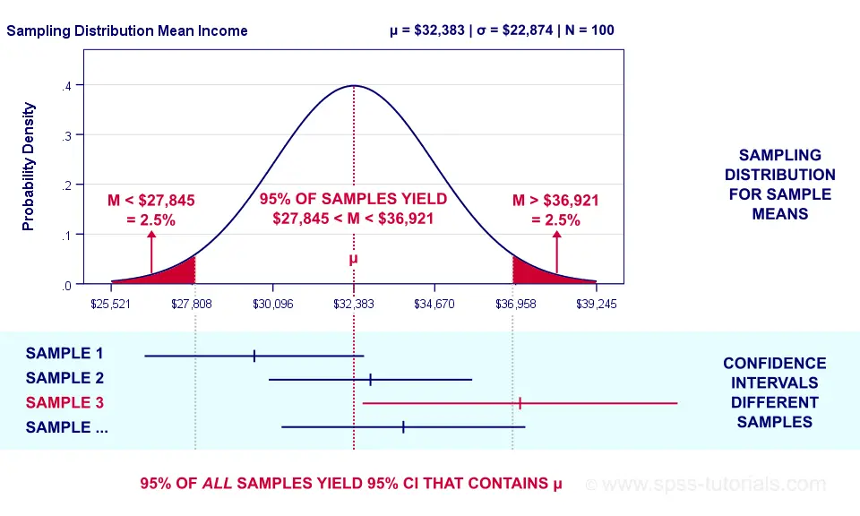
https://www.spss-tutorials.com/confidence-intervals/
흔히 우리가 가지고 있는 표본을 통해 추정한 구간 안에 모평균이 존재할 확률이 95% 라고 말하곤 하는데 이것은 잘못된 해석입니다.
모평균의 구간추정#
모분산을 알고 있는 경우
신뢰 구간을 추청하는 방식을 이용하면 모분산(\(\sigma^2\))을 알고 있을 경우, 모평균의 95% 신뢰 레벨(Confidence Level) 또는 5% 유의 수준(Significance Level, \(\alpha\))을 가지는 신뢰 구간(Confidence Interval)을 표준화하여 표준정규분포상에서 아래와 추정 할 수 있게 됩니다.
\(\mathsf{\text{Confidence Interval (z-score)} = \left[ \bar{x} - z_{\alpha/2} \times \frac{\sigma}{\sqrt{n}}, \bar{x}+z_{\alpha/2} \times \frac{\sigma}{\sqrt{n}} \right]}\)
\(\alpha/2\): Significance level for two-tailed, \(\frac{\sigma}{\sqrt{n}}\): Standard error for population
\(\bar{X} - z_{0.025} \times \frac{\sigma}{\sqrt{n}} \leq \mu \leq \bar{X} + z_{0.025} \times \frac{\sigma}{\sqrt{n}}\)
\(\bar{X} - 1.96 \times \frac{\sigma}{\sqrt{n}} \leq \mu \leq \bar{X} + 1.96 \times \frac{\sigma}{\sqrt{n}}\)
# 모집단(Population): 평균 1.0 과 분산 2.0 의 정규분포
p_mean = 1.0
p_var = 2.0
p_std = np.sqrt(p_var)
# 정규분포 연속 확률 변수 (Normal continuous random variable)
rv = sp.stats.norm(loc=p_mean, scale=np.sqrt(p_var))
print(f"population: p_mean={p_mean}, p_var={p_var}")

# 표본(Sample): 10개의 데이터를 가지는 표본을 랜덤 샘플링
size = 30
# 무작위 표본, 랜덤 변량 (Random variates)
samples = rv.rvs(size)
print(f"sample: samples.shape={samples.shape}")

# 신뢰구간 (confidence level), 유의수준 (significance level)
cl = .95
sl = (1.-cl)/2 # for Two-Tailed (양측검정)
print(f"estimation: cl={cl}, sl={sl:.3f}")

# 표본평균(Sample Mean), 모분산(Population Variance), 표준오차(Standard Error)
s_mean = np.mean(samples)
p_ste = p_std / np.sqrt(size)
# 신뢰구간 하한 (Lower confidence limit), 신뢰구간 상한 (Upper confidence limit)
# 경계값 (Critical Value)
z_cv = sp.stats.norm.ppf(1.-sl)
lcl = s_mean - z_cv * p_ste
ucl = s_mean + z_cv * p_ste
print(f"estimation: lcl={lcl:.5f} <= p_mean={p_mean} <= ucl={ucl:.5f}")

# interval 함수 이용
lcl, ucl = sp.stats.norm.interval(alpha=cl, loc=s_mean, scale=p_ste)
print(f"estimation: lcl={lcl:.5f} <= p_mean={p_mean} <= ucl={ucl:.5f}")
population: p_mean=1.0, p_var=2.0
sample: samples.shape=(30,)
estimation: cl=0.95, sl=0.025
estimation: lcl=0.19276 <= p_mean=1.0 <= ucl=1.20488
estimation: lcl=0.19276 <= p_mean=1.0 <= ucl=1.20488
모분산을 모르는 경우
하지만, 일반적으로 모집단의 분산을 모르기때문에, 모집단이 정규분포를 따른다른 가정하에 n-1의 자유도를 따르는 t 분포 및 표본분산(\(s^2\))를 이용하여 모평균의 신뢰 구간을 추정할 수 있습니다. t 분포는 표본 수가 적어도 사용 가능하며, 표본 수가 충분히(30 이상) 크면 정규 분포와 거의 같아지므로 작은 표본에서도 사용할 수 있습니다. t 분포에서 95% 신뢰 구간은 아래와 같이 추정할 수 있게 됩니다.
\(\mathsf{\text{Confidence Interval (t-score)} = \left[ \bar{x} - t_{\alpha/2}(n-1) \times \frac{s}{\sqrt{n}}, \bar{x}+t_{\alpha/2}(n-1) \times \frac{s}{\sqrt{n}} \right]}\)
\(\alpha/2\): Significance level for two-tailed, \(\frac{s}{\sqrt{n}}\): Standard error for sample
\(\bar{X} - t_{0.025}(n-1) \times \frac{s}{\sqrt{n}} \leq \mu \leq \bar{X} + t_{0.025}(n-1) \times \frac{s}{\sqrt{n}}\)
t 분포의 경우 표본 수가 확률에 영향을 미치므로, 예로 n = 10 이라고 한다면, 아래와 같습니다.
\(\bar{X} - 2.26 \times \frac{s}{\sqrt{n}} \leq \mu \leq \bar{X} + 2.26 \times \frac{s}{\sqrt{n}}\)
# 모집단(Population): 평균 1.0 과 분산 2.0 의 정규분포
p_mean = 1.0
p_var = 2.0
# 정규분포 연속 확률 변수 (Normal continuous random variable)
rv = sp.stats.norm(loc=p_mean, scale=np.sqrt(p_var))
print(f"population: p_mean={p_mean}, p_var={p_var}")

# 표본(Sample): 30개의 데이터를 가지는 표본을 랜덤 샘플링
size = 30
# 무작위 표본, 랜덤 변량 (Random variates)
samples = rv.rvs(size)
print(f"sample: samples.shape={samples.shape}")

# 신뢰구간 (confidence level), 유의수준 (significance level), 자유도 (Degree of Freedom)
cl = .95
sl = (1.-cl)/2 # for Two-Tailed (양측검정)
dof = size - 1 # Degree of Freedom
ddof = 1 # Delta Degrees of Freedom (dof = n - ddof)
print(f"estimation: cl={cl}, sl={sl:.3f}, ddof={ddof}")

# 표본평균(Sample Mean), 표본편차(Sample Standard Deviation) , 표준오차 (Standard Error)
s_mean = np.mean(samples)
s_std = np.std(samples)
s_ste = s_std / np.sqrt(size)
# 신뢰구간 하한 (Lower confidence limit), 신뢰구간 상한 (Upper confidence limit)
# 경계값 (Critical Value)
t_cv = abs(sp.stats.t.ppf(sl, dof))
lcl = s_mean - t_cv * s_ste
ucl = s_mean + t_cv * s_ste
print(f"estimation: lcl={lcl:.5f} <= p_mean={p_mean} <= ucl={ucl:.5f}")

# interval 함수 이용
lcl, ucl = sp.stats.t.interval(alpha=cl, df=dof, loc=s_mean, scale=s_ste)
print(f"estimation: lcl={lcl:.5f} <= p_mean={p_mean} <= ucl={ucl:.5f}")
population: p_mean=1.0, p_var=2.0
sample: samples.shape=(30,)
estimation: cl=0.95, sl=0.025, ddof=1
estimation: lcl=0.47725 <= p_mean=1.0 <= ucl=1.61852
estimation: lcl=0.47725 <= p_mean=1.0 <= ucl=1.61852
모분산의 구간추정#
모분산의 신뢰 구간은 표본분산과 비례하는 \(x^2\) 분포를 따르며, 95% 신뢰 구간을 아래와 같이 추정이 가능합니다.
\(\mathsf{\text{Confidence Interval} (x^2) = \left[ \frac{(n-1)s^2}{x^2_{\alpha/2}(n-1)}, \frac{(n-1)s^2}{x^2_{1-\alpha/2}(n-1)} \right]}\)
\(\alpha/2\): Significance level for two-tailed
\(\frac{(n-1)s^2}{x^2_{0.025}(n-1)} \leq \sigma^2 \leq \frac{(n-1)s^2}{x^2_{0.975}(n-1)}\)
\(\frac{(n-1)s^2}{11.143} \leq \sigma^2 \leq \frac{(n-1)s^2}{0.484}\)
# 모집단(Population): 평균 1.0 과 분산 2.0 의 정규분포
p_mean = 1.0
p_var = 2.0
# 정규분포 연속 확률 변수 (Normal continuous random variable)
rv = sp.stats.norm(loc=p_mean, scale=np.sqrt(p_var))
print(f"population: p_mean={p_mean}, p_var={p_var}")

# 표본(Sample): 30개의 데이터를 가지는 표본을 랜덤 샘플링
size = 30
# 무작위 표본, 랜덤 변량 (Random variates)
samples = rv.rvs(size)
print(f"sample: samples.shape={samples.shape}")

# 신뢰구간 (confidence level), 유의수준 (significance level), 자유도 (Degree of Freedom)
cl = .95
sl = (1.-cl)/2 # for Two-Tailed (양측검정)
dof = size - 1 # Degree of Freedom
ddof = 1 # Delta Degrees of Freedom (dof = n - ddof)
print(f"estimation: cl={cl}, sl={sl:.3f}, ddof={ddof}")

# 표본평균(Sample Mean), 표본편차(Sample Standard Deviation) , 표준오차 (Standard Error)
s_mean = np.mean(samples)
s_var = np.var(samples, ddof=ddof)
# 신뢰구간 하한 (Lower confidence limit), 신뢰구간 상한 (Upper confidence limit)
# 경계값 (Critical Value)
c2_cv_l = sp.stats.chi2.ppf(1.-sl, dof)
c2_cv_u = sp.stats.chi2.ppf(sl, dof)
lcl = (size - 1) * s_var / c2_cv_l
ucl = (size - 1) * s_var / c2_cv_u
print(f"estimation: lcl={lcl:.5f} <= p_var={p_var} <= ucl={ucl:.5f}")
population: p_mean=1.0, p_var=2.0
sample: samples.shape=(30,)
estimation: cl=0.95, sl=0.025, ddof=1
estimation: lcl=1.63014 <= p_var=2.0 <= ucl=4.64470
베르누이 분포의 모평균의 구간추정#
지금까지는 모집단이 정규분포를 따르는 경우에 대한 신뢰구간에 대한 계산 이었습니다. 하지만 모집단이 정규분포를 따르지 않을 경우에도 표본 평균의 분포는 정규분포를 따른다는 ‘중심극저한정리’를 이용하면, 신뢰구간 추정이 가능합니다.
제품의 인지도, 후보의 득표율, 프로그램의 시청율 등 확률변수가 1/0을 가지는 모집단의 비율을 추정하고 싶을 경우, 이 표본은 베르누이 확률분포를 따르지만, 표본의 평균은 정규분포에 근사하기 때문에, 이 정규분포를 표준화 하여 아래와 같이 신뢰 구간 추정을 할 수 있습니다.
\(\mathsf{\text{Confidence Interval} (Bern) = \left[ \bar{X}-z_{\alpha/2}\sqrt{\bar{X}(1-\bar{X})/n}, \bar{X}-z_{1-\alpha/2}\sqrt{\bar{X}(1-\bar{X})/n} \right]}\)
\(\alpha/2\): Significance level for two-tailed
# 제품 호감도 조사 샘플: 선호:1, 비선호:0
samples = [1, 0, 1, 1, 1, 1, 1, 0, 1]
size = len(samples)

# 신뢰구간 (confidence level), 유의수준 (significance level), 자유도 (Degree of Freedom)
cl = .95
sl = (1.-cl)/2 # for Two-Tailed (양측검정)
print(f"estimation: cl={cl}, sl={sl:.3f}")

s_mean = np.mean(samples)
# 신뢰구간 하한 (Lower confidence limit), 신뢰구간 상한 (Upper confidence limit)
# 경계값 (Critical Value)
cv_l = sp.stats.norm.ppf(1.-sl)
cv_u = sp.stats.norm.ppf(sl)
lcl = s_mean - cv_l * np.sqrt(s_mean*(1-s_mean)/size)
ucl = s_mean - cv_u * np.sqrt(s_mean*(1-s_mean)/size)
print(f"estimation: lcl={lcl:.5f}, ucl={ucl:.5f}")
estimation: cl=0.95, sl=0.025
estimation: lcl=0.50617, ucl=1.04939
포아송 분포의 모평균의 구간추정#
단위 시간당 발생하는 건수와 같은 포아송 분포 또한 표본평균은 중심극한정리에 따라 정규분포를따르기 때문에 표준정규분포로 표준화하여 아래와 같이 신뢰구간을 추정할 수 있습니다.
\(\mathsf{\text{Confidence Interval} (Poi) = \left[ \bar{X}-z_{\alpha/2}\sqrt{\bar{X}/n}, \bar{X}-z_{1-\alpha/2}\sqrt{\bar{X}/n} \right]}\)
\(\alpha/2\): Significance level for two-tailed
#시간당 사이트 접속자 수
samples = [12, 10, 4, 7, 6, 5, 50, 1, 7]
size = len(samples)

# 신뢰구간 (confidence level), 유의수준 (significance level), 자유도 (Degree of Freedom)
cl = .95
sl = (1.-cl)/2 # for Two-Tailed (양측검정)
print(f"estimation: cl={cl}, sl={sl:.3f}")

s_mean = np.mean(samples)
# 신뢰구간 하한 (Lower confidence limit), 신뢰구간 상한 (Upper confidence limit)
# 경계값 (Critical Value)
cv_l = sp.stats.norm.ppf(1.-sl)
cv_u = sp.stats.norm.ppf(sl)
lcl = s_mean - cv_l * np.sqrt(s_mean/size)
ucl = s_mean - cv_u * np.sqrt(s_mean/size)
print(f"estimation: lcl={lcl:.5f}, ucl={ucl:.5f}")
estimation: cl=0.95, sl=0.025
estimation: lcl=9.13393, ucl=13.53274